Predicting Adult Income: An End-to-End Machine Learning Pipeline Project

This project demonstrates a complete machine learning workflow using the Adult Income dataset to predict whether a person earns more than $50K annually. It begins with exploratory data analysis (EDA) using Seaborn to uncover key patterns and relationships in the data. A custom transformer is developed to engineer a new feature which captures how education and weekly working hours interact to influence income potential. The project then builds a scikit-learn data pipeline that handles preprocessing, encoding, feature scaling, and model training. Three models: Logistic Regression, Support Vector Machine (SVM), and Random Forest, are trained and evaluated using cross-validation, with Logistic Regression emerging as the most efficient and interpretable performer. The result is a clean, reproducible workflow that highlights practical data analysis, feature engineering, and model evaluation skills.

Imports

import numpy as np
import pandas as pd
import matplotlib.pyplot as plt
import seaborn as sns

from sklearn.model_selection import train_test_split, cross_val_score, GridSearchCV, cross_validate
from sklearn.pipeline import Pipeline, make_pipeline
from sklearn.compose import ColumnTransformer
from sklearn.preprocessing import OneHotEncoder, StandardScaler, OrdinalEncoder
from sklearn.impute import SimpleImputer
from sklearn.base import BaseEstimator, TransformerMixin
from sklearn.feature_selection import SelectKBest, mutual_info_classif
from sklearn.linear_model import LogisticRegression
from sklearn.ensemble import RandomForestClassifier
from sklearn.svm import SVC
from sklearn.metrics import (
    accuracy_score, precision_score, recall_score, f1_score,
    roc_auc_score, confusion_matrix, classification_report, RocCurveDisplay
)
from sklearn.feature_selection import SelectKBest, mutual_info_classif

import warnings
warnings.filterwarnings('ignore')

Data Loading and Initial Inspection

df = pd.read_csv("C:\\Users\\misul\\Data\\adult.csv")
df.head()

Data Cleaning

#Basic cleaning: strip whitespace and replace '?' as NaN (if needed)
for c in df.select_dtypes(include='object').columns:
    df[c] = df[c].str.strip()
df.replace('?', np.nan, inplace=True)

df.isna().sum().sort_values(ascending=False)

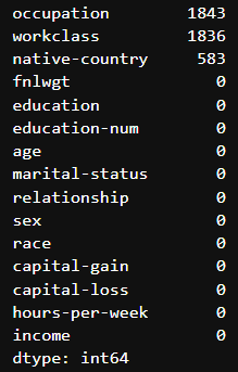
df.dropna(inplace=True)
df.isna().sum().sort_values(ascending=False)

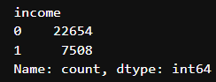
# Ensure target is binary 0/1
df['income'] = df['income'].map({'<=50K': 0, '<=50K':0, '>50K':1, ' >50K':1, '>-50K':1, '> 50K':1}).astype(int)
df['income'].value_counts()

Exploratory Data Analysis (EDA) and Visualization

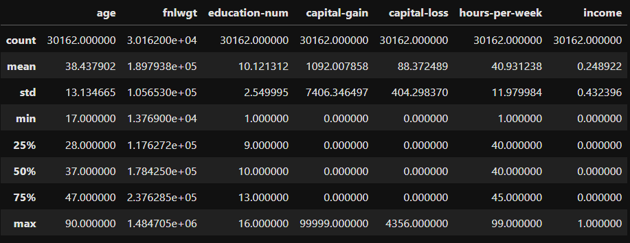
df.describe()

plt.rcParams['figure.figsize'] = (20, 10)
sns.set(font_scale=1)

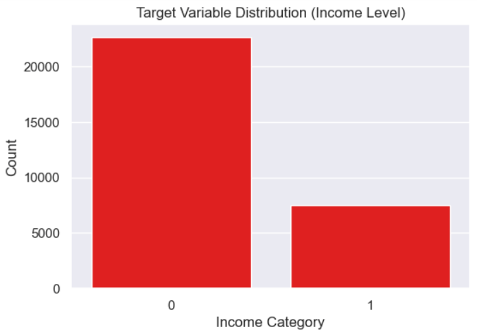
plt.figure(figsize=(6,4))
sns.countplot(x='income', data=df, color='red')
plt.title("Target Variable Distribution (Income Level)")
plt.xlabel("Income Category")
plt.ylabel("Count")
plt.show()

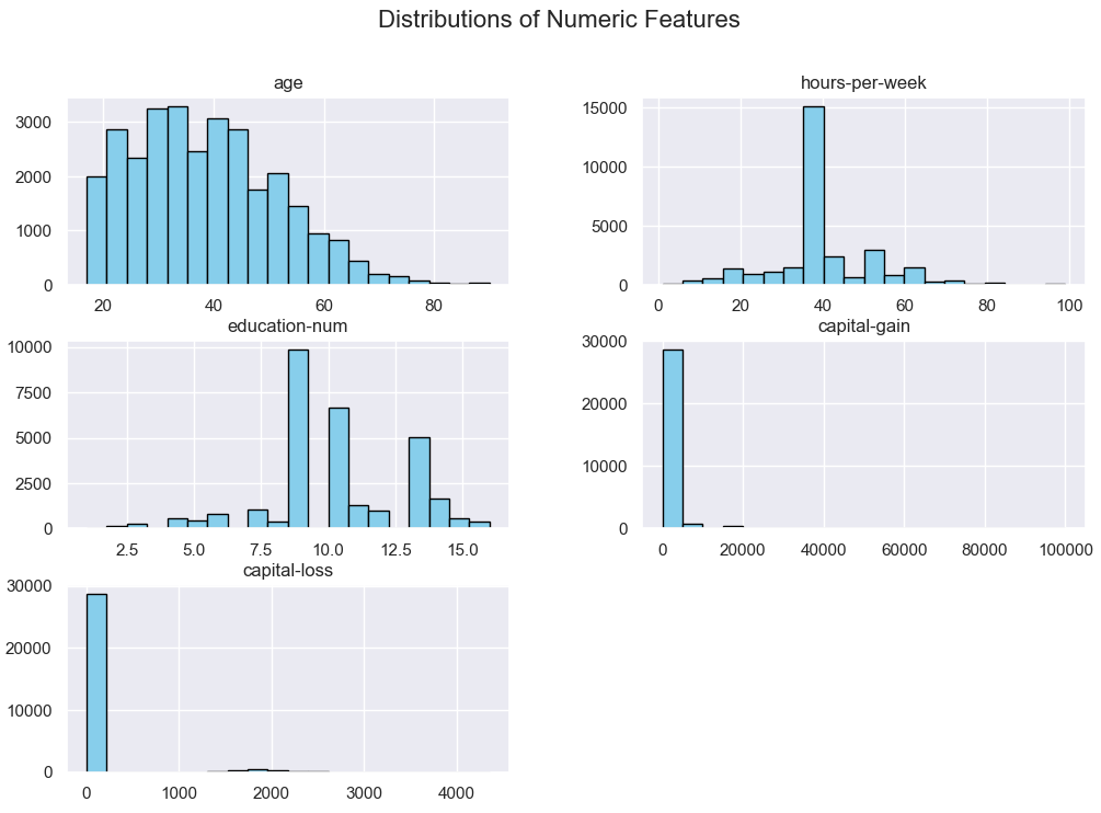
numeric_features = ['age', 'hours-per-week', 'education-num', 'capital-gain', 'capital-loss']

df[numeric_features].hist(bins=20, figsize=(12,8), color='skyblue', edgecolor='black')
plt.suptitle("Distributions of Numeric Features", fontsize=16)
plt.show()

plt.figure(figsize=(6,4))
sns.boxplot(x='income', y='age', data=df, color='purple')
plt.title("Age vs. Income")
plt.show()

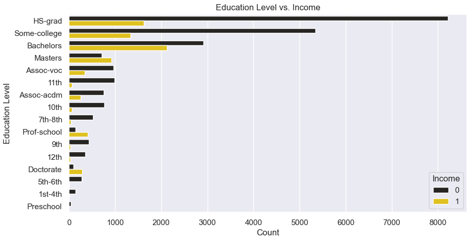
plt.figure(figsize=(10,5))
sns.countplot(y='education', hue='income', data=df, order=df['education'].value_counts().index, color='gold')
plt.title("Education Level vs. Income")
plt.xlabel("Count")
plt.ylabel("Education Level")
plt.legend(title='Income')
plt.show()

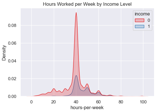
plt.figure(figsize=(6,4))
sns.kdeplot(data=df, x='hours-per-week', hue='income', fill=True, palette='Set1')
plt.title("Hours Worked per Week by Income Level")
plt.show()

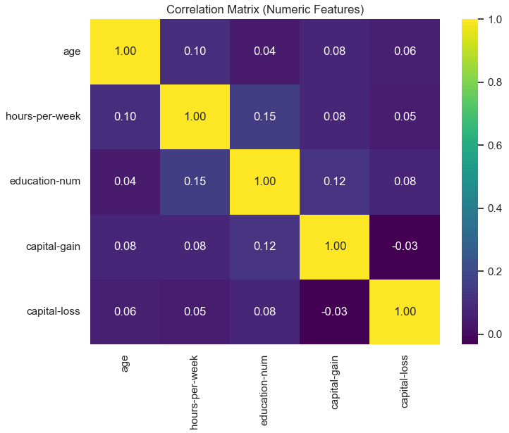
plt.figure(figsize=(8,6))
corr = df[numeric_features].corr()
sns.heatmap(corr, annot=True, cmap="viridis", fmt=".2f")
plt.title("Correlation Matrix (Numeric Features)")
plt.show()

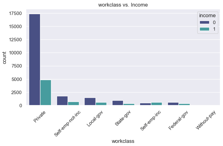
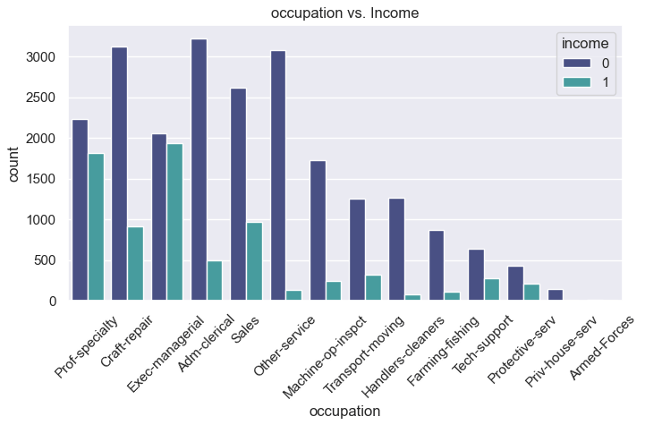
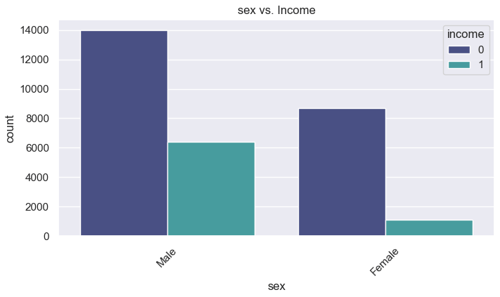
categorical_features = ['workclass', 'marital-status', 'occupation', 'sex']

for col in categorical_features:
    plt.figure(figsize=(8,4))
    sns.countplot(x=col, hue='income', data=df, order=df[col].value_counts().index, palette='mako')
    plt.title(f"{col} vs. Income")
    plt.xticks(rotation=45)
    plt.show()

Create the Custom Transformer

# Custom Transformer: WorkloadTransformer
# This will add a categorical column 'workload_level' based on hours-per-week.

class WorkloadTransformer(BaseEstimator, TransformerMixin):
    """
    Transform hours-per-week into a categorical workload_level:
      - part-time: <= 30
      - standard: 31-40
      - long-hours: 41-60
      - excessive: >60
    Returns the original DataFrame with an added column 'workload_level'.
    """
    def __init__(self, hours_col='hours-per-week', new_col='workload_level'):
        self.hours_col = hours_col
        self.new_col = new_col

    def fit(self, X, y=None):
        # nothing to learn
        return self

    def transform(self, X):
        X = X.copy()
        if not isinstance(X, pd.DataFrame):
            X = pd.DataFrame(X, columns=[self.hours_col])
        bins = [0, 30, 40, 60, np.inf]
        labels = ['part-time', 'standard', 'long-hours', 'excessive']
        X[self.new_col] = pd.cut(X[self.hours_col], bins=bins, labels=labels, include_lowest=True)
        return X

Preprocessing and Pipeline Setup

# Features to use - drop fnlwgt (not informative), keep both education and education-num optionally
drop_cols = ['fnlwgt']  # or you can drop more
target = 'income'

# Let's decide features to include
feature_cols = [c for c in df.columns if c not in [target] + drop_cols]

# Split before pipeline to keep test set clean
X = df[feature_cols].copy()
y = df[target].copy()

X_train, X_test, y_train, y_test = train_test_split(
    X, y, test_size=0.2, stratify=y, random_state=42
)

# Columns by type
numeric_features = ['age', 'education-num', 'capital-gain', 'capital-loss', 'hours-per-week']
categorical_features = [c for c in feature_cols if c not in numeric_features]

# Preprocessing for numeric
numeric_transformer = Pipeline(steps=[
    ('imputer', SimpleImputer(strategy='median')),
    ('scaler', StandardScaler())
])

# Preprocessing for categorical
categorical_transformer = Pipeline(steps=[
    ('imputer', SimpleImputer(strategy='most_frequent')),
    ('onehot', OneHotEncoder(handle_unknown='ignore', sparse_output=False))
])

# Assemble ColumnTransformer
preprocessor = ColumnTransformer(transformers=[
    ('num', numeric_transformer, numeric_features),
    ('cat', categorical_transformer, categorical_features)
], remainder='drop', verbose_feature_names_out=False)

Full Pipeline with Custom Transformer and a Classifier

# Pipeline with logistic regression (baseline)
pipeline_logreg = Pipeline([
    ('workload', WorkloadTransformer(hours_col='hours-per-week', new_col='workload_level')),
    # Now we add workload_level to categorical features - we'll update ColumnTransformer to reflect that below.
])

# Update categorical_features to include workload_level if it isn't already
if 'workload_level' not in categorical_features:
    extended_categorical = categorical_features + ['workload_level']
else:
    extended_categorical = categorical_features

# New preprocessor using workload_level
preprocessor_extended = ColumnTransformer(transformers=[
    ('num', numeric_transformer, numeric_features),
    ('cat', Pipeline(steps=[
        ('imputer', SimpleImputer(strategy='most_frequent')),
        ('onehot', OneHotEncoder(handle_unknown='ignore', sparse_output=False))
    ]), extended_categorical)
], remainder='drop', verbose_feature_names_out=False)

# Final pipeline
pipeline_logreg = Pipeline([
    ('workload', WorkloadTransformer(hours_col='hours-per-week', new_col='workload_level')),
    ('preproc', preprocessor_extended),
    ('clf', LogisticRegression(max_iter=1000, solver='liblinear'))
])

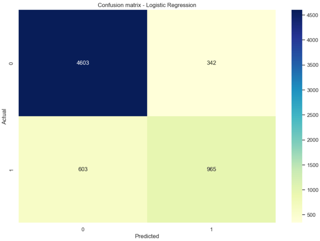
Train Baseline Logistic Regression Model and Evaluate

pipeline_logreg.fit(X_train, y_train)
y_pred = pipeline_logreg.predict(X_test)
y_proba = pipeline_logreg.predict_proba(X_test)[:,1]

print("Logistic Regression (baseline) metrics:")
print("Accuracy:", accuracy_score(y_test, y_pred))
print("Precision:", precision_score(y_test, y_pred))
print("Recall:", recall_score(y_test, y_pred))
print("F1:", f1_score(y_test, y_pred))
print("ROC AUC:", roc_auc_score(y_test, y_proba))
print("\nClassification report:\n", classification_report(y_test, y_pred))

# Confusion matrix visualization
sns.set(font_scale=1)
plt.figure(figsize=(12,8))
cm = confusion_matrix(y_test, y_pred)
sns.heatmap(cm, annot=True, fmt='d', cmap='YlGnBu')
plt.xlabel('Predicted')
plt.ylabel('Actual')
plt.title('Confusion matrix - Logistic Regression')
plt.show()

Feature Selection

# Feature selection using SelectKBest (mutual_info_classif) applied AFTER preprocessing ===
# We need a pipeline that exposes the numeric + one-hot features to SelectKBest.
# Approach: Preprocess the data then run SelectKBest within a pipeline before classifier.

# Pipeline with feature selection
pipeline_fs = Pipeline([
    ('workload', WorkloadTransformer(hours_col='hours-per-week', new_col='workload_level')),
    ('preproc', preprocessor_extended),
    ('select', SelectKBest(score_func=mutual_info_classif, k=20)),  # choose k
    ('clf', RandomForestClassifier(n_estimators=200, random_state=42))
])

# Fit and evaluate with cross-validation
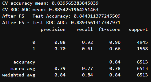
cv_results = cross_validate(pipeline_fs, X_train, y_train, cv=5, scoring=['accuracy','roc_auc'], return_train_score=False)
print("CV accuracy mean:", cv_results['test_accuracy'].mean())
print("CV ROC AUC mean:", cv_results['test_roc_auc'].mean())

# Fit to train and evaluate on holdout test
pipeline_fs.fit(X_train, y_train)
y_pred_fs = pipeline_fs.predict(X_test)
y_proba_fs = pipeline_fs.predict_proba(X_test)[:,1]

print("After FS - Test Accuracy:", accuracy_score(y_test, y_pred_fs))
print("After FS - Test ROC AUC:", roc_auc_score(y_test, y_proba_fs))
print(classification_report(y_test, y_pred_fs))

def get_feature_names_from_preprocessor(preprocessor, numeric_features, categorical_features):
    feature_names = []
    # numeric
    feature_names.extend(numeric_features)
    # categorical - get categories from OneHotEncoder
    cat_pipeline = preprocessor.transformers_[1][1]  # the Pipeline we made for categorical
    onehot = cat_pipeline.named_steps['onehot']
    # If we used a pipeline with imputer then onehot
    # Get categories
    for i, col in enumerate(categorical_features):
        cats = onehot.categories_[i]
        feature_names.extend([f"{col}__{c}" for c in cats])
    return feature_names

# preprocessor_extended has our categorical pipeline as second transformer
feature_names_full = get_feature_names_from_preprocessor(preprocessor_extended, numeric_features, extended_categorical)
selected_mask = pipeline_fs.named_steps['select'].get_support()
selected_features = [name for name, sel in zip(feature_names_full, selected_mask) if sel]
print("Selected features (k=20):", selected_features)

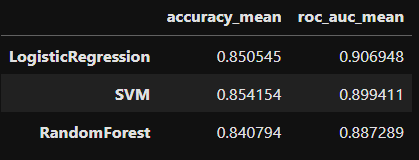
Comparing Models: Logistic Regression, Random Forests, and Support Vector Machines

models = {
    'LogisticRegression': Pipeline([
        ('workload', WorkloadTransformer(hours_col='hours-per-week', new_col='workload_level')),
        ('preproc', preprocessor_extended),
        ('clf', LogisticRegression(max_iter=1000, solver='liblinear'))
    ]),
    'RandomForest': Pipeline([
        ('workload', WorkloadTransformer(hours_col='hours-per-week', new_col='workload_level')),
        ('preproc', preprocessor_extended),
        ('clf', RandomForestClassifier(n_estimators=200, random_state=42))
    ]),
    'SVM': Pipeline([
        ('workload', WorkloadTransformer(hours_col='hours-per-week', new_col='workload_level')),
        ('preproc', preprocessor_extended),
        ('clf', SVC(kernel='rbf', probability=True, random_state=42))
    ])
}

results = {}
for name, model in models.items():
    scores = cross_validate(model, X_train, y_train, cv=3, scoring=['accuracy','roc_auc'])
    results[name] = {
        'accuracy_mean': scores['test_accuracy'].mean(),
        'roc_auc_mean': scores['test_roc_auc'].mean()
    }

pd.DataFrame(results).T.sort_values('roc_auc_mean', ascending=False)

# Here I'm going to tune the hyperparameters for the SVM model for demonstration purposes only
# The Logistic Regression model will be used because it performed the best
# The Random Forest model did not perform as well as the SVM model so I will not tune hyperparameters for that one. 

param_grid_svm = {
    'clf__C': [0.1, 1, 10],
    'clf__gamma': ['scale', 'auto'],
    'clf__kernel': ['linear', 'rbf']
}

svm_pipeline = models['SVM']
gs_svm = GridSearchCV(svm_pipeline, param_grid_svm, cv=3, scoring='roc_auc', n_jobs=-1)
gs_svm.fit(X_train, y_train)
print("Best params for SVM:", gs_svm.best_params_)
print("Best CV ROC AUC:", gs_svm.best_score_)

y_pred_svm = gs_svm.predict(X_test)
y_proba_svm = gs_svm.predict_proba(X_test)[:, 1]
print("Test ROC AUC:", roc_auc_score(y_test, y_proba_svm))

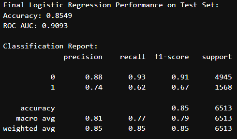
Refit Logistic Regression Model, Make Predictions, and Evaluate

# Refit Logistic Regression pipeline on the entire training data
final_model = models['LogisticRegression']
final_model.fit(X_train, y_train)

# Make predictions on the test set
y_pred = final_model.predict(X_test)
y_pred_proba = final_model.predict_proba(X_test)[:, 1]

# Evaluate performance
test_accuracy = accuracy_score(y_test, y_pred)
test_auc = roc_auc_score(y_test, y_pred_proba)

print("Final Logistic Regression Performance on Test Set:")
print(f"Accuracy: {test_accuracy:.4f}")
print(f"ROC AUC: {test_auc:.4f}")
print("\nClassification Report:")
print(classification_report(y_test, y_pred))

# visualize ROC curve
RocCurveDisplay.from_estimator(final_model, X_test, y_test)